
Toolbox Table of Contents
- Biodiversity estimates: species richness, weighted endemism and corrected weighted endemism
- Landscape connectivity
- Commonly used ArcMap Tools
- SDM Tools: MaxEnt:
- Modeling with MaxEnt
- Correcting latitudinal background selection bias:
- Distribution changes between binary SDMs:
- Background Selection via bias files:
- Over-prediction correction: clip models by buffered minimum convex polygons
- SDM Tools: Universal:
- Create friction layer: invert SDMs
- Split binary SDM by input clade relationship
- Explore Climate Data
- Limit dispersal in future SDMs
- Distribution changes between binary SDMs
- Spatially Rarefy Occurrence Data for SDMs (reduce spatial autocorrelation)
- Microclim Tools
- Create Microclim Bioclim variable – single factor
- Create Microclim Bioclim variable – two factors
- Over-prediction correction: clip models by buffered minimum convex polygons
- Shapefile and table tools:
- Raster tools:
- Batch extract by mask (by folder)
- Batch raster to ASCII (by folder)
- Batch ASCII to raster (by folder)
- Batch NetCDF to raster (by folder)
- Batch raster to raster (by folder)
- Batch project raster to equal-area projection (by folder)
- Batch project raster to any projection (by folder)
- Batch define projection as WGS1984
- Batch resample grids (by folder)
- Batch upscale grids (by folder)
- Batch sum rasters – any extent (by folder)
- Batch sum rasters- all same extent (by folder)
- Apply same color ramp to all open rasters
- Export JPEGs of all open files
- Export images of all color permutations of RGB raster
- Quick reclassify to binary
- Quick reclassify
- Batch reclassify (by folder)
- Correlation and summary Stats
- Zonal statistics of many rasters to single table
- Project Shapefiles to User Specified Projection (folder)
- Define Projection (folder)
- Polygon to Raster (folder)
- NetCDF to Raster (folder)
- Define NoData Value (folder)
- Advance Upscale Grids (folder
- Export JPEGs of all open files
- Sample raster values at input localities (folder)
- Increase Raster Extent/Snap All Raster to Same Extent (folder)
- Raster Calculator: Plus (Folder)
- Raster Calculator: Subtract (Folder)
- Raster Calculator: Times (Folder)
- Raster Calculator: Divide (Folder)
- Raster Calculator: Standardize 0-1 (Folder)
- Multiband NetCDF to Separate Rasters
- Multiband NetCDF to Separate Rasters (Folder)
- Advance Downscale Grids (Folder)
Commonly Used ArcMap Tools
This is a convenient grouping of 23 existing Spatial Analyst tools within ArcGIS 10 that are commonly used for geospatial analyses in ecology and evolution studies (i.e. Raster Calculator and Reclassify). For legacy ArcGIS users, this familiar grouping of functions is almost identical to the tools contained in the Spatial Analysis Toolbar (now absent from ArcMap 10). Because these tools are well documented within the software and are not novel, they are not discussed in detail here, see ESRI.
Biodiversity Analyses
These tools estimate three common biodiversity metrics: species richness, weighted endemism and corrected weighted endemism. There are two sets of analyses here. Analyses that utilize point occurrence data and analyses that use binary SDMs. As follows are the three diversity metrics: 1. Species Richness (SR) is sum of unique species per cell.
SR = K (the total number of species in a grid cell)
2. Weighted Endemism (WE), which is the sum of the reciprocal of the total number of cells each species in a grid cell is found in. A WE emphasizes areas that have a high proportion of animals with restricted ranges.
WE = ∑ 1/C (C is the number of grid cells each endemic occurs in)
3. Corrected Weighted Endemism (CWE). The corrected weighted endemism is simply the weighted endemism divided by the total number of species in a cell (Crisp 2001). A CWE emphasizes areas that have a high proportion of animals with restricted ranges, but are not necessarily areas that are species rich.
CWE = WE/K (K is the total number of species in a grid cell)
Crisp, M. D., Laffan, S., Linder, H. P., and Monro, A. 2001. Endemism in the Australian flora. Journal of Biogeography 28:183-198. 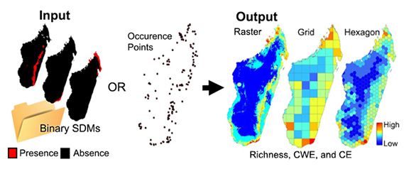
CANAPE categorization
Runs categorizations of neo- and paleo-endemism on grids output from Biodiverse
Quickly reclassify significance from randomizations
Uses data from Biodiverse to randomize and reclassify significance
Landscape Connectivity
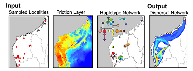
Least-Cost Corridors and Least-Cost Paths: Haplotype Network
This tool creates a raster of the sum of least-cost corridors and a polyline shapefile of least-cost paths between populations that share haplotypes. Often a single LCP between sites oversimplifies landscape processes. By using categories of cost paths that include paths with slightly more costly path lengths (relative to the LCP), you can better depict habitat heterogeneity and its varying roles in dispersal. For each comparison you can classify the lowest cost paths into three categories. Lastly, a density analysis will produce a raster depicting the frequency that LCPs traverse the same path. For more information, see: Chan LM, Brown JL, Yoder AD (2011). Integrating statistical genetic and geospatial methods brings new power to phylogeography. Mol Phylogenet Evol 59(2):523-537.
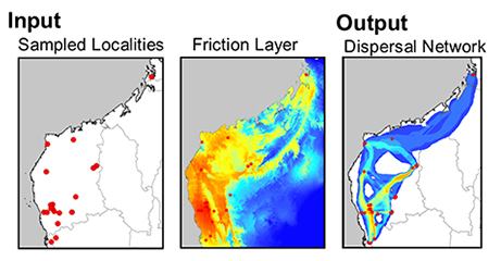
Least-Cost Corridors and Least-Cost Paths: Pairwise Comparison
This tool creates a raster of the sum of least-cost corridors and a polyline shapefile of least-cost paths between all populations. Often a single LCP between sites oversimplifies landscape processes. By using categories of cost paths that include paths with slightly more costly path lengths (relative to the LCP), you can better depict habitat heterogeneity and its varying roles in dispersal. For each comparison you can classify the lowest cost paths into three categories. Lastly, a density analysis will produce a raster depicting the frequency that LCPs traverse the same path.
Create Pairwise Distance Matrix
This tool will create two pair-wise distance matrices reflecting: least-cost path distance and the along path cost (of each least-cost path). The least-cost path distance is simply the distance of the LCP. The along path cost (of the least-cost path) is the total sum of the friction values that characterize the least-cost path. Each output is a n-dimensional symmetrical matrix output as a CSV table.
Split SDM by input Clade relationship- Inverse Distance Weighting
This script uses a set of species distribution models and a set of points for intraspecific lineages to generate lineage distribution models. VERY IMPORTANT: column headings for species/group ID and lineage/clade ID must be 12 characters or less. Also input models must be a TIFF raster (.tif) and perfectly match species/group name in CSV table. See example data.
If you use this tool, in addition to citing SDMtoolbox, please cite the researchers who developed this really cool method:
Rosauer DF, Catullo RA, VanDerWal J, Moussalli A, Hoskin CJ, Moritz C (2015) Lineage Range Estimation Method Reveals Fine-Scale Endemism Linked to Pleistocene Stability in Australian Rainforest Herpetofauna. PLoS ONE 10(5): e0126274.
MaxEnt Tools
Run MaxEnt: Spatial Jackknifing
This tool executes the MaxEnt modeling application (http://www.cs.princeton.edu/~schapire/maxent/).
Why use SDMtoolbox for MaxEnt analyses:
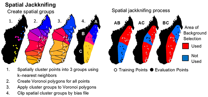
I. Spatial Jackknifing
Spatial jackknifing (or geographically structured k-fold cross-validation) tests evaluation performance of spatially segregated spatially independent localities. SDMtoolbox automatically generates all the GIS files necessary to spatially jackknife your MaxEnt Models. The script splits the landscape into 3-5 regions based on spatial clustering of occurrence points (e.g, for 3 regions: A,B,C). Models are calibrated with k-1 spatial groups and then evaluated with the withheld group. For example if k=3, then models would be run with following three subgroups:
-
-
- Model is calibrated with localities and background points from region AB and then evaluated with points from region C
- Model is calibrated with localities and background points from region AC and then evaluated with points from region B
- Model is calibrated with localities and background points from region BC and then evaluated with points from region A
-
II. Independent Tests of Model Feature Classes and Regularization Parameters
Equally important, this tool allows for testing different combinations of five model feature class types (FC) and regularization multipliers (RM) to optimize your MaxEnt model performance. For example, if a RM was input (here 5), this tool kit would run MaxEnt models on the following parameters for each species:
-
-
- RM: 5 & FC: Linear
- RM: 5 & FC: Linear and Quadratic
- RM: 5 & FC: Hinge
- RM: 5 & FC: Linear, Quadratic and Hinge
- RM: 5 & FC: Linear, Quadratic, Hinge, Product and Threshold
-
III. Automatic Model Selection
Finally, the script chooses the best model by evaluating each model’s: 1. omission rates (OR)*,2. AUC**, and 3. model feature class complexity. It does this in order, choosing the model with the lowest omission rates on the test data. If many models have the identical low OR, then it selects the model with the highest AUC. Lastly if several models have the same low OR and high AUC, it will choose the model with simplest feature class parameters in the following order(1. linear; 2. linear and quadratic; 3. hinge; 4. linear, quadratic, and hinge; and 5. linear, quadratic, hinge, product, and threshold).
Once the best model is selected, SDMtoolbox will run the final model using all the occurrence points. If desired, at this stage models will be projected into other climates, environmental variables will be jackknifed to measure importance, and response curves will be created.
*For each iteration, OR is weighted by the number of points in the evaluation subgroup. This is necessary because spatial groups may not have identical number of points. The weighing gives equal contribution to all points included in model evaluation.
**AUC is calculated from the total study area in the input bias file (groups ABC)
For info and justification for each of these methods see:
Boria, R. A., L. E. Olson, S. M. Goodman, and R. P. Anderson. 2014. Spatial filtering to reduce sampling bias can improve the performance of ecological niche models. Ecological Modelling, 275:73-77.
Radosavljevic, A. and R. P. Anderson. 2014. Making better Maxent models of species distributions: complexity, overfitting, and evaluation. Journal of Biogeography. 41:629-643
Shcheglovitova, M. and R. P. Anderson. 2013. Estimating optimal complexity for ecological niche models: a jackknife approach for species with small sample sizes. Ecological Modelling, 269:9-17.
Hack the output batch files to make them do exactly what you want!
If SDMtoolbox doesn’t do everything you want for your modeling project, good news: many changes are easy to implement in the output batch code yourself (post-GIS).
I want to:
Keep all ASCII outputs: Open the ‘Step1_Optimize_MaxEnt_Model_Parameters.bat’ file in a text editor. If modeling a single species, delete the second last line (it ends in “DeleteASCIIs.py”). E.g. start C:\Python27\ArcGIS10.1\pythonw.exe C:\Users\Jason\Desktop\Maxent\outfolder\Furcifer_oustaleti\GISinputs\DeleteASCIIs.py If modelling more species, find all lines referencing the “DeleteASCIIs.py” and delete them. Alternate: simply delete the “DeleteASCIIs.py” file from the GISinputs folder for each species.
Spatially jackknife and output the final ‘best models’ as raw (not logistic): Run ‘Step1’, then open the ‘Step2_Run_Optimized_MaxEnt_Models.bat’ file in a text editor. Search and replace ‘ -a’ with ‘ outputformat=raw -a’. Then find the ‘”applythresholdrule=…” section, search and replace: “applythresholdrule=minimum training presence” (or whatever yours actually is) with “”.
Run more then one final model (e.g. the top five models) : Open the ‘FinalRank.py’ file in a text file located in the GISinputs folder (in each species folder). Also open the “.._SUMSTATS_RANKED_MODEL.csv” file and note the pairs of regularization numbers and feature ID number that you want to run in final models. Go back to the ‘FinalRank.py’ file and page down ca. 25 lines, find the “If RegN==X and FeatN==Y:” that matche your regularization number (X) and feature ID number (Y) pairs. Copy the text inside the quotes in the following line, after the text ‘resA=’. Paste that in the next line of the ‘Step2_Run_Optimized_MaxEnt_Models.bat’ file. Lastly, be sure to change output location, which follows the ‘-o’ in the code. Else models will successively overwrite each other. Alternate: run each one at a time (simply saving batch code in text file with “.bat” as extension), then move them from standard output ‘final’ folder to a new appropriately named folder.
Automatically test many regularization multipliers and different feature class combinations, but not spatially jackknife. To do this, check ‘spatial jackknifing’ but then change the minimum number of points to spatially jackknife to ‘100000’. Assuming you have less than 100000 occurrence records, all species will be run according to the parameters under the heading ‘Model Parameters for Species Not Spatially Jackknifed’.
Is there a hack you would like help with, perhaps I can help? Do you have a spatial jackknife batch file hack? Please consider contributing it for others. Email me and I may post it here.
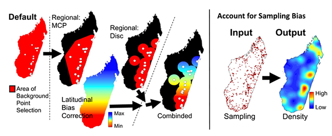
Correcting Latitudinal Background Selection Bias
If you are using data that are in a geographic coordinate systems (such as, degrees minutes seconds or decimal degrees) for MaxEnt analyses (and most other psuedoabsence based SDM methods)— then you are biasing your selection of background/pseudoabsences and unique observed localities toward the poles. The level of bias depends on the breadth of latitudes your analyses cover. The reason for this is due to the area occupied by these units decreases latitudinally (as values increase, see Table 1) and areas are largest at equator and smallest at poles. This inequality results from convergence of the meridians (lines of longitude) towards the poles. There are two solutions to this issue. The first issue address corrects the bias sampling problem by correcting how pseudo-absence values and unique occurrence localities are selected. The second solution fixes the problem by projected all the data into an equal-areas projection (EAP). The latter is the preferred method, however for many modelers this requires considerable effort and can be confusing due to issues associated with selecting the best EAP. The SDM toolbox facilitates both solutions. The first set of tools clips a Coordinate Bias File to the size of your MaxEnt analysis and then calculates a BFCD for that area. The Coordinate Bias File accounts for background/pseudo-absence sampling biases associated with latitudinal changes in the area encompassed by decimal degree units. This tool converts the Coordinate Bias File to the proportion of area occupied (relative to the largest value present in your analyses) to be used as a bias file in MaxEnt. A value of 2 in the output file depicts a 50% reduction in cell area (vs. cell values of 1). Thus, in absence of a BFCD, the probability of creating background point in the cell with a value of 2 is twice as high as a cell with a value of 1. The BFCD allows equal sampling of background points throughout the landscape in geographic projections.
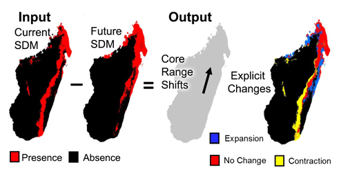
Distribution Changes Between Binary SDMs
A common use of species distribution models is to predict distributional changes due to climate change. Here we created two tools that help summarize distributional changes. The first tool calculates the distributional changes between two binary SDMs (e.g. current and future SDMs). Output is a table depicting the km2 of range contraction, range expansion and no change in the species distribution. A second tool also calculates the distributional changes between two binary SDMs (e.g. current and future SDMs), however this analysis is focused on summarizing the core distributional shifts in many species’ ranges. This analysis reduces each species’ distribution to a single central point (a centroid) and creates a vector file depicting magnitude and direction of change through time.
Limit Species’ Dispersal in Future SDMs
A common use of species distribution models is to predict distributional changes due to future climate change. This tool sets dispersal limitations between current and future SDMs.This tool clips future SDMs by a maximum dispersal distance from the current presence predicted area . This removes future suitable habitat that is too far from currently predicted suitable habitat– those areas not likely to be dispersed into. 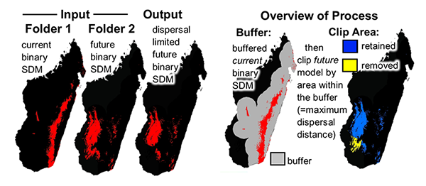
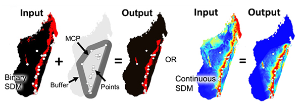
Overprediction Correction: Clip Models by Buffered Minimum Convex Polygons
To limit over-prediction of SDMs, a problem common with modeling species distributions, we created two tools that clip SDMs by a buffered minimum convex polygon (MCP) generated from the input point data of each species following the approach of Kremen et al. (2008). This method produces models that represent suitable habitat within an area of known occurrence (based on a buffered MCP), excluding suitable habitat greatly outside of observed range and unsuitable habitat through the landscape.
Kremen, C., A. Cameron, A. Moilanen, S. J. Phillips, C. D. Thomas, H. Beentje, J. Dransfield, B. L. Fisher, F. Glaw, T. C. Good, G. J. Harper, R. J. Hijmans, D. C. Lees, E. Louis Jr., R. A. Nussbaum, C. J. Raxworthy, A. Razafimpahanana, G. E. Schatz, M. Vences, D. R. Vieites & M. L. Zjhra (2008): Aligning conservation priorities across taxa in Madagascar with high-resolution planning tools. – Science 320: 222-226.
Background Selection via Bias Files
A subset of tools create bias files used to fine-tune background and occurrence point selection in Maxent. Bias files control where background points are selected and the density of background sampling. This avoids sampling habitat greatly outside of a species’ known occurrence or can account for both collection sampling biases and latitudinal biases associated with coordinate data. Typically background points are selected within a large rectilinear area, within this area there often exist habitat that is environmentally suitable, but was never colonized. When background points are selected within these habitats, this increases commission errors (false-positives) and subsequently results in the ‘best’ performing model to be over-fit, favoring a model that doesn’t predict the species in the un-colonized suitable habitat (Anderson & Raza 2010, Barbet-Massin et al. 2012).
Background points (and similar pseudo-absence points) are meant to be compared with the presence data and help differentiate the environmental conditions under which a species can potentially occur. However when the background is sampled too far from the species’ realized distribution, these points can be sampled from climatically suitable, unoccupied habitats that were never colonized to due considerable unsuitable habitat in between. The likelihood of sampling suitable unoccupied habitats increases with Euclidean distance from current range of the species. Thus, a larger study spatial extent can lead to the selection of a higher proportion of less informative background points (Barbet-Massin et al. 2012). This does not mean researchers should avoid studying species with broad distributions or those existing in regions that do not conform well to rectilinear map layouts (that results in many background points selected from unoccupied suitable habitat), rather they simply need to be more selective in the choice of background points in MaxEnt (and pseudo-absences in other SDM methods).
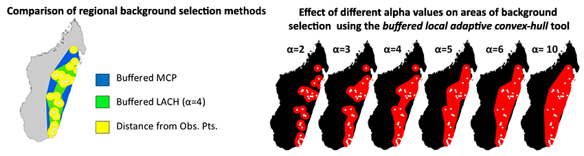
To circumvent this problem many researchers have begun using background point and pseudo-absence selection methods that are more regional. SDMtoolbox contains two tools to facilitate more sophisticated background selection for use in Maxent. The Sample by Distance from Obs. Pts. tool uses a common method that samples backgrounds within a maximum radial distance of known occurrences (see Thuiller et al. 2009). The Sample by buffered MCP tool restricts background selection with a buffered minimum-convex polygons based on known occurrences. The Sample by buffered local adaptive convex-hull tool restricts background selection to an intermediate area of the latter two tools. One limitation of presence-only data SDM methods is the effect of sample selection bias from sampling some areas of the landscape more intensively than others (Phillips et al. 2009).
Maxent requires an unbiased sampling of occurrence data and spatial sampling biases can be reduced by using the Gaussian kernel density of sampling localities tool. This method produces a bias grid that up-weights presence-only data points with fewer neighbors in the geographic landscape. To do this the tool creates a Gaussian kernel density of sampling localities. Output bias values of 1 reflect no sampling bias, whereas higher values represent increased sampling bias. Depending on the study, the input points could be all sampling localities for a larger taxonomic group or simply the input sampling localities of a focal species. For example, if I were studying a single species of frog from Madagascar, I could use either: 1) only the occurrence points from that species, or 2) all sampling points from all amphibians in Madagascar. The former focuses on sampling biases in the focal species, where the latter focuses on widespread spatial sampling biases and likelihood of detection of your species in all surveys (e.g. sampling only near roads).
Anderson, R. P. & Raza, A. (2010) The effect of the extent of the study region on GIS models of species geographic distributions and estimates of niche evolution: preliminary tests with montane rodents (genus Nephelomys) in Venezuela. Journal of Biogeography, 37, 1378-1393.
Barbet-Massin, M., Jiguet, F., Albert, C. H. & Thuiller, W. (2012) Selecting pseudo-absences for species distribution models: how, where and how many? Methods in Ecology and Evolution, 3, 327–338.
Phillips, S.J., Dudík, M., Elith, J., Graham, C.H., Lehmann, A., Leathwick, J. & Ferrier, S. (2009) Sample selection bias and presence‐only distribution models: implications for background and pseudo‐absence data. Ecological Applications, 19,181–197.
Thuiller, W., Lafourcade, B., Engler, R. & Araujo, M. B. (2009) BIOMOD – a platform for ensemble forecasting of species distributions. Ecography, 32, 369–373.
Universal SDM Tools
Create Friction Layer: Invert SDM
The use of least-cost paths and along-path distances often dramatically improve the calculation of geographic distance for testing hypotheses (such as, isolation by distance). However few studies have access to meaningful friction landscapes. Some researchers (i.e. Broquet et al. 2006) generate friction landscapes from classified satellite images— where each major habitat type represents a different value. A primary downfall to using habitat heterogeneity as a friction landscape is the weighing of each habitat class to represent relevant friction values. Doing this properly relies heavily on expert life history knowledge and when done analyses loses some objectivity. For example, Broquet et al. (2006) adjusted the friction values until they satisfied prior expectations. More recently authors used LCP and species distribution models (SDMs) as friction landscapes (Wang et al. 2008, Chan et al 2011). This method is a more objective alternative to expert knowledge and the generation of high quality SDMs can be done with relative ease for many species.
Broquet, T., Ray, N., Petit, E., Fryxell, J.M. & Burel, F. (2006) Genetic isolation by distance and landscape connectivity in the american marten (martes americana). Landscape Ecology, 21, 877-889
Chan LM, Brown JL, Yoder AD (2011). Integrating statistical genetic and geospatial methods brings new power to phylogeography. Mol Phylogenet Evol 59(2):523-37.
Wang, Y.H., Yang, K.C., Bridgman, C.A., Lin, L.K. (2008) Habitat suitability modelling to correlate gene flow with landscape connectivity. Landscape Ecology, 23, 989–1000 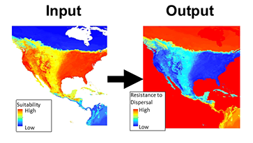
Explore Climate Data: Correlation and Summary Stats
This tool calculates summary statistics (mean, maximum, minimum and standard deviation) for each input raster layer. This tool also calculates correlation and covariance coefficients of each input raster to all other included rasters (output is in the form of a matrix).
Explore Climate Data: Remove highly correlated variables
This tool evaluates the correlations among all input environment data and then removes layers that are correlated at the user specified level. Layers that you wish to retain (vs. the other correlated layers) should be first in the list. All correlated layers that occur after will be excluded. For interpreting influence of environmental layers in the SDM, I prefer to place layers that depict metrics frequently used in non-SDM ecology and evolution studies (see a few listed below). Further for simplicity, these layers often best represent the original input climate data (as they directly reflect the actual measurements) and are not derived from several layers or a subset of the data.
BIO1 = Annual Mean Temperature
BIO2 = Mean Diurnal Range (Mean of monthly (max temp – min temp))
BIO12 = Annual Precipitation
Note1: this tool uses the absolute values of the correlation coefficient (vs. a signed coefficient)
Note2: All input rasters must have the same NoData value (e.g. -9999 from signed 16bit rasters)
Distribution Changes Between Binary SDMs
A major use of species distribution models is to predict distributional changes due to future climate change. Here we created two tools that help summarize distributional changes. The first tool calculates the distributional changes between two binary SDMs (e.g. current and future SDMs). Output is a table depicting the km2 of range contraction, range expansion and no change in the species distribution. A second tool also calculates the distributional changes between two binary SDMs (e.g. current and future SDMs), however this analysis is focused on summarizing the core distributional shifts in many species’ ranges. This analysis reduces each species’ distribution to a single central point (a centroid) and creates a vector file depicting magnitude and direction of change through time.
Limit Species’ Dispersal in Future SDMs
A common use of species distribution models is to predict distributional changes due to future climate change. This tool sets dispersal limitations between current and future SDMs.This tool clips future SDMs by a maximum dispersal distance from the current presence predicted area . This removes future suitable habitat that is too far from currently predicted suitable habitat– those areas not likely to be dispersed into.
Overprediction Correction: Clip Models by Buffered Minimum Convex Polygons
To limit over-prediction of SDMs, a problem common with modeling species distributions, we created two tools that clip SDMs by a buffered minimum convex polygon (MCP) generated from the input point data of each species following the approach of Kremen et al. (2008). This method produces models that represent suitable habitat within an area of known occurrence (based on a buffered MCP), excluding suitable habitat greatly outside of observed range and unsuitable habitat through the landscape.
Kremen, C., A. Cameron, A. Moilanen, S. J. Phillips, C. D. Thomas, H. Beentje, J. Dransfield, B. L. Fisher, F. Glaw, T. C. Good, G. J. Harper, R. J. Hijmans, D. C. Lees, E. Louis Jr., R. A. Nussbaum, C. J. Raxworthy, A. Razafimpahanana, G. E. Schatz, M. Vences, D. R. Vieites & M. L. Zjhra (2008): Aligning conservation priorities across taxa in Madagascar with high-resolution planning tools. – Science 320: 222-226.
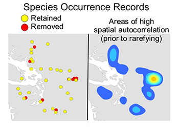
Rarify Occurence Data for SDMs (reduce spatial autocorrelation)
This tool removes spatially autocorrelated occurrence points by reducing multiple occurrence records to a single record within the specified distance. For most SDM methods to perform well, they require input occurrence data to be spatially independent. It is common for researchers to introduce environmental biases into their SDMs from spatially autocorrelated input occurrences. This causes SDMs to be over-fit towards environmental bias resulting from sampling bias introduced from spatially clustered occurrences. The elimination of spatial clusters of localities is important for model calibrating and model evaluation. When spatial clusters of localities exist, models often are over-fit (reducing the model’s ability to predict spatially independent data) and model performance values are inflated. The spatially rarefy occurrence data tool addresses this issue by spatially filtering locality data by a user input distance, reducing occurrence localities to a single point within the specified Euclidian distance. This tool also allows users to spatially rarefy their data at several distances according to habitat, topographic or climate heterogeneity (Table 1d). For example, occurrence localities could be spatially filtered at 5 km2, 10 km2 and 30 km2 in areas of high, medium and low environmental heterogeneity, respectively. This graduated filtering method is particular useful for studies with limited occurrence points and can maximize the number of spatially independent localities. Three additional tools calculate climate and topographic heterogeneity for rarefying at multiple distances. The climate heterogeneity tool calculates the first three principal components (PCs) of all input climate data. Then it calculates the heterogeneity of each PC, weighs each PC heterogeneity layer by the amount of variation explained, and sums them to produce the final heterogeneity layer. Input point data must be in the WGS 1984 geographic coordinate system.
Shapefile and Table Tools
CSV, TXT, XLS to Shapefile
This tool converts a CSV, TXT, or XLS spreadsheet with latitude and longitude to a point shapefile.
Shapefile to CSV
This tool converts a point shapefile to CSV spreadsheet with latitude and longitude.
Randomly select points
This tool randomly select a subset of points.
Split shapefile by fields
This tool splits a shapefile into several by unique field ID.
Create tessellated hexagons of a region
This tool creates regular hexagons tessellated across the defined study area.
Sample raster or feature values to hexagons
This tool samples raster values to coarser tessellated hexagons. It does this by sampling all the raster values contained within each hexagon. The manner that it samples rasters depends on the type of zonal statistic used (click ‘zonal statistic type’ menu for explanation of all the available statistics). For example, if the raster depicts a continuous variable then the ‘mean’ or ‘median’ statistics might be good options. Alternatively, if the raster depicts non-ordered categories, than ‘majority’ might be a better choice. Output values are appended to input hexagon shapefile with a single value depicting each hexagon.
Batch project shapefile to any projection (by folder)
This tool projects a folder of shapefiles to any specified projection.
Define projection as WGS84 (by folder)
This tool will define the projection of all GIS layers in a folder to WGS1984.
Raster Tools
Batch extract by mask (by folder)
This tool clips a folder of rasters (such as climate data) to a smaller area by mask, coordinates or map extent. See user guide for overview of how to prepare Worldclim climate date for use in Maxent.
Batch raster to ASCII (by folder)
This tool converts a folder of rasters to ASCII rasters.
Batch ASCII to raster (by folder)
This tool converts a folder of ASCII rasters to another raster format.
Batch NetCDF to raster (by folder)
This tool converts a folder of NetCDF rasters to another raster format.
Batch raster to raster (by folder)
This tool converts a folder of rasters (.tif, .img, .bil, .bip, .bmp, .bsq, .dat, .gif, .jpg, .jp2, .png) to another raster format (.tif, .img, .bil, .bip, .bmp, .bsq, .dat, .gif, .jpg, .jp2, .png).
Batch project raster to equal-area projection (by folder)
This tool projects a folder of WGS 1986 projected rasters to a equal-area projection.
Batch project raster to any projection (by folder)
This tool projects a folder of rasters to any specified projection.
Define projection as WGS84 (by folder)
This tool will define the projection of all GIS layers in a folder to WGS1984.
Batch resample grids (by folder)
This tool resamples a folder of rasters to any resolution.
Batch upscale grids (by folder)
Upscales all grids in a folder (upscales = to coarser resolution).
Batch sum rasters – any extent (by folder)
This tools sums all raster in a folder. Note rasters can be of any extent.
Batch sum rasters- all same extent (by folder)
This tools sums all raster in a folder.
Apply same color ramp to all open rasters
This tools applies the same color ramp to all open rasters.
Export Images of All Color Permutation of a RGB raster
For choosing the best color scheme, this tool will export images of all permutations of red, green and blue of a 3-band raster.
Export JPEGs of all open files
This tool will export JPEGs of all open files as view from extent of the map viewer.
Quick reclassify to binary
This tool quickly reclassifies a raster to a binary raster. Simply input the cutoff threshold.
Quick reclassify
This tool quickly reclassifies a raster to user specified values. Simply input the cutoff ranges.
Batch reclassify (by folder)
This tool quickly reclassifies all rasters in a folder to the same user specified values.
Correlation and Summary Stats
This tool calculates summary statistics (mean, maximum, minimum and standard deviation) for each input raster layer. This tool also calculates correlation and covariance coefficients of each input raster to all other included rasters (output is in the form of a matrix).
Zonal statistics of many rasters to single table
Calculates statistics on values of a raster within the zones of another dataset. This tool will calculate zonal stats of a folder rasters and then merge all the results to a single table.
Project Shapefiles to User Specified Projection (folder)
Projects entire folder of shapefiles to any input projection
Define Projection (folder)
Use to define the projection of any input (shapefile or raster)
Polygon to Raster (folder)
Converts polygon input into a raster format
NetCDF to Raster (folder)
Converts all NetCDF (.nc) files to raster
Define NoData Value (folder)
Redefines NoData value in rasters. Used to fix an error when creating rasters where the NoData value is changed
Advance Upscale Grids (folder)
Upscales all grids in folder to a coarser resolution
Export JPEGs of all open files
Exports JPEGS of all files in the map viewer
Sample raster values at input localities (folder)
Samples the values of TIFF rasters at the locations input. Allows field names to be up to 50 characters
Increase Raster Extent/Snap All Raster to Same Extent (folder)
This tool will increase or decrease spatial extent of all input rasters